DEA – A brief introduction
Data Envelopment Analysis is a state of the art benchmarking technique which is particularly useful for multi-criteria benchmarking studies. In DEA, the productivity of a unit is evaluated by comparing the amount of output(s) produced in comparison to the amount of input(s) used. The performance of a unit is calculated by comparing its efficiency with the best observed performance in the data set. There exist many different DEA models, each with its own characteristics. This page will however concentrate on the main concepts of DEA.
A bit of history
Early performance measurement used to principally focus on financial output performance disregarding other areas (such as production or customer service) or ignoring the concept of efficiency. The consequences of this omission prompted econometricians to rethink how conventional econometric analysis looked at production functions and how it dealt with variations in efficiency [1].
Production functions, which model the structure of production, have been developed and refined over more than 80 years (e.g. by Cobb and Douglas [2]). However, Kumbhakar and Knox Lovell [3] point out that while conventional econometrics tends to use production, cost, and profit functions, they assume that producers allocate inputs and outputs efficiently and that producers operate on these functions apart from randomly distributed statistical noise. The authors state anecdotal evidence (p. 2) which suggests that producers are not always successful in solving their optimisation problems efficiently. This can be illustrated by inefficiently utilising the resources (inputs) in the production process (this is called technical inefficiency (Cooper et al., 2007)), or by poorly allocating resources and production targets (this is called mix inefficiency [4]. Producers not solving their optimisation problem correctly were consequently not operating on the production functions used, up to then, to measure performance.
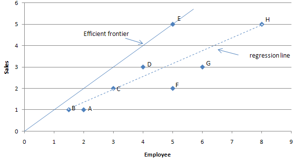
In the light of the clear limitations of traditional production functions, productivity analysis’ focus moved towards production frontiers. The literature that directly influenced the development of frontier analysis methods began in the 1950’s with the work of Koopmans [5] who mentioned that a producer would be efficient ‘if, and only if, it is impossible to produce more of any output without producing less of some other output or using more of some input’. Koopmans’ original work prompted Debreu in 1951 [6] and Shephard (1953 [7] cited in [8]) to develop models which associated the distance function with technical efficiency. This work was critical to the development of further literature on efficiency. Farrell (1957) [9] applied for the first time these developments to measure technical efficiency in an agricultural context. This innovative work influenced the creation of two major frontier analysis techniques: Stochastic Frontier Analysis (SFA) and Data Envelopment Analysis (DEA). The concept of efficient frontier is illustrated in the figure below for a one input, one output case. The best performers are on the frontier line (in this case the best performer is E).
Farrell’s paper (1957) – which did not correctly address mix inefficiencies[10] – prompted Charnes, Cooper and Rhode (CCR, 1978[11]) to develop another frontier analysis method called Data Envelopment Analysis (DEA). DEA is a non-parametric benchmarking method (i.e. which does not use statistical distribution) which measures productivity by considering a system of inputs and outputs. Since this paper, many different Data Envelopment Analysis models have been introduced (e.g. BCC, SBM, ADD or FDH [12], some being drastically different from this original model and DEA has become a well established performance measurement technique.
Efficiency ratio
Efficiency is the ratio between the outputs produced with the amount of inputs used. The ‘volume of sales per employee’, the ‘GDP per capita’, or the ‘average number of passenger per flight’ are common example of efficiency ratio. DEA measures the efficiency of a unit (called Decision Making Units or DMU) using a weighted ration as illustrated below:
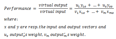
The ratio above accounts for all outputs and inputs. This type of measure is called Total Productivity Factor. All DEA models implement similar type of performance ratios although with their own specific characteristics. The weights assigned to each input and each output are variables used in the DEA optimisation process.
Efficient frontier
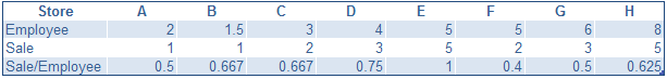
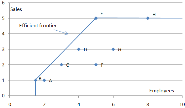
The efficient frontier represents the best observed performance in the data set. The concept is best explained with a simple example. Let’s consider the following table showing number of employees and sales figures for some food stores. The efficiency ratio (sales / employee) can be used to measure the efficiency of the different stores The table is as follows:
Plotting this data with employees on the x axis (the horizontal axis), and the sales on the y axis (the vertical axis) will give the following graph:
The table and graph allows to find the best performers. In this case, store E shows the best performance with an efficiency of 1. The line that spans from the origin to store E is the efficiency frontier. The efficiency frontier illustrates the best observed performance and is said in mathematics to ‘envelop’ the data; hence DEA’s name. The region enveloped by the efficient frontier is called the Production Possibility Set. This is the region of possible production (based on the observed best performance).
In DEA, the performance of a DMU is always calculated by comparing it to the efficiency frontier directly determined from the data.
Becoming efficient
All the DMU that are not on the efficiency frontier are inefficient (a DMU on the efficiency frontier is not necessarily efficient but this point is discussed here with DMU H situation). An inefficient unit must consequently reach the efficiency frontier in order to become efficient. There are three possibilities:
- Reduce the inputs while keeping the outputs constant (this is an input oriented approach),
- Increase the outputs while keeping the inputs constant (this is an output orientated approach).
- Both increasing outputs while reducing the inputs (this can be done with non-oriented versions of models such as the SBM model).
In effect, the further away from the frontier an entity is, the worse its performance.
This can be illustrated by considering DMU C from the previous graph:
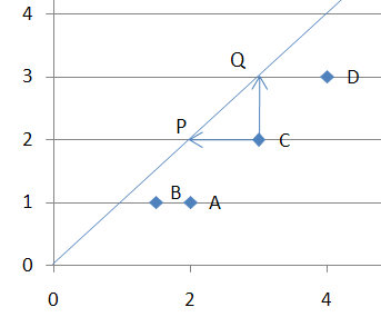
This illustration shows how DMU C can either reach the frontier by reducing its inputs (whilst keeping its output levels constant) and reach ‘P’, or by increasing its output (whilst keeping its input levels constant) and reach Q.
Returns to scale
It is important to note that the frontier pictures in the graphs above is assumed to stretch to infinity; i.e. that the performance levels of DMU E (the only efficient store) are possible regardless of the number of employee the store has. This is called Constant returns to scale (Constant RTS). Although the constant RTS assumption is sometimes true for a local range of production, it sometimes need to be relaxed. This is possible with – for example – variable returns to scale which are illustrated in the graph below:
Note that under variable returns to scale, DMU B becomes efficient.
Although DMU H is on the efficiency frontier, it is not efficient. This is caused by DMUE which produces a similar amount of ‘sales’ (i.e. 5) but uses 3 less units of ’employees’ to do so. In order for H to be efficient, it will need to reduce its sales force by 3 employees in order to reach E’s coordinates. DMUH could also become efficient by increasing its sales. However there is no way to know for sure if this is possible as such production levels have not been observed (i.e. above the current efficiency frontier).
There exist other types of Returns to Scale such as Increasing Returns To Scale (sometimes also called Non Decreasing Returns To Scale, e.g. by Seiford and Zhu[13]) which assume that it is not possible to reduce the scale of DMU but that RTS can strech to infinity. Another type of RTS which is the he opposite assumption to IRTS is the Decreasing Returns To Scale (also sometimes called non-increasing RTS). Finally, there is a General RTS model that allows to control how much the scale of DMU can be reduced or increased.
Technical & Mix Inefficiencies
There exist two types of inefficiency:
- Technical inefficiency
- Mix inefficiencies
The difference between the two can be best explained with a simple example. The following graph illustrates the performance of different vehicles depots based on 2 outputs: utilisation and sales, and one input: number of vehicles. It is possible to illustrate the performance of each depot by plotting the utilisation/vehicle and the sales/vehicle ratio values. This is illustrated below:
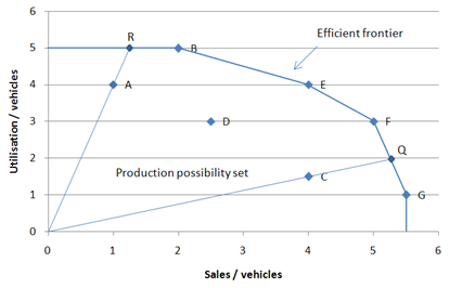
On this graph, DMU C is not efficient as it is not on the efficiency frontier (see Becoming efficient above). In order for DMU C to become efficient, it needs to reach the frontier by projecting on to Q. This radial projection corresponds to the technical inefficiency of DMU C. DMU A is also not efficient as not on the efficient frontier. However, when projecting on the efficient frontier to R (technical inefficiencies), DMU A is still not efficient as there exist another DMU (DMU B) which illustrates proportionally greater sales output per vehicles. In order for DMU A to become efficient, it first needs to project on to the efficiency frontier and then increase it sales per vehicle output until it reaches B (mix inefficiencies). The amount of improvement between Q and B is measured by the non-negative slack of A on its sales performance.
Technical inefficiencies can thus be eliminated without changing the proportions between inputs and outputs while mix inefficiencies can only be eliminated by changing the proportion (mix) between inputs and outputs. DEA models have different approaches as to how the technical and mix inefficiencies are evaluated. DMUs are efficient when they exhibit no technical inefficiencies and no mix inefficiencies.
Reference Set / Peers
In the graph above, Q, the projections of DMU C on the efficient frontier, is between DMU F and DMU G. DMU F and DMU G are called the Reference Set of DMU C. The reference set of a given DMU consists of the list of efficient DMUs which performance was used to calculate the efficiency of the given DMU.
How does DEA work?
As explained earlier, DEA uses a total factor productivity ratio to measure performance (i.e. a unique ratio with all the inputs and outputs). DEA attributes a virtual weight tp each of these input and output.
Entities’ performance is then calculated using a linear optimisation process which tries to maximise each entity’s ratio by finding the best set of weight for this particular entity.
The optimisation process is contrained by existing data so that each entity is compared against the best observed performance.
This simple example should have introduced most of DEA’s basic concepts. Although the example only used a single input and a single output, DEA is more useful when performance needs to take multiple inputs and outputs into account. More information specific to different DEA models (e.g. CCR, BCC, SBM) will be made available on this site correspondingly to the library releases.
References
- ↑ Kumbhakar Subal C., Lovell Knox, Stochastic Frontier Analysis, Cambridge University Press, 2000, p. 1
- ↑ Cobb C.W., Douglas, P.H., A Theory of Production, American Economic Review, Vol. 18 (Supplement), pp. 139-165
- ↑ Kumbhakar Subal C., Lovell, Knox, Stochastic Frontier Analysis, Cambridge University Press, 2000, p. 1
- ↑ Cooper William W., Seiford Lawrence M., Tone Karou Data Envelopment Analysis – A Comprehensive Text with Models, Applications References and DEA-Solver Software. Second Edition, Springer, 2007
- ↑ Koopmans Tjalling, C., Activity Analysis of Production and Allocation, Activity Analysis of Production and Allocation Conference, John Wiley & Sons Inc – Chapman & Hall, 1951
- ↑ Debreu G., The Coefficient of Resource Utilization, The Econometric Society, 1951, Vol. 19, Issue 3, pp. 273-292
- ↑ Shepard R.W., Cost and Production Functions, Princeton University Press, 1953
- ↑ Kumbhakar Subal C., Lovell, Knox, Stochastic Frontier Analysis, Cambridge University Press, 2000, p. 7
- ↑ Farrell M.J., The Measurement of Productive Efficiency, Journal of the Royal Statistical Society. Series A (General), Blackwell Publishing for the Royal Statistical Society, Vol.120, Issue 3, pp. 253-290
- ↑ Cooper, William W.; Seiford, Lawrence M.; Tone Karou Data Envelopment Analysis – A Comprehensive Text with Models, Applications References and DEA-Solver Software. Second Edition, Springer, 2007, pp. 46-47
- ↑ Charnes, A.; Cooper, W.W.; Rhodes, E. Measuring the efficiency of decision making units. European Journal of Operational Research, 1978, Vol. 2, p. 429.
- ↑ Cooper, William W.; Seiford, Lawrence M.; Tone Karou Data Envelopment Analysis – A Comprehensive Text with Models, Applications References and DEA-Solver Software. Second Edition, Springer, 2007
- ↑ Seiford L.M., Zhu J., An investigation of returns to scale in data envelopment analysis, International Journal of Management Science, Vol. 27, 1999, pp. 1-11
External Links
This section lists a few links to different web sites of potential interest. The order in which the sites are listed does not reflect any preference of any kind.
Further Information
Further information on DEA can be found at the following links:
- Wikipedia DEA web page.
- The deazone web site.
- The OR-Notes web page from J. E. Beasley.
- The DEA Online Software web site.
Some DEA software
Here is a list of some DEA software:
- The Performance Improvement Management software (PIM) developped under the supervision of Prof. Emmanual Thanassoulis and of Dr Ali Emrouznejad.
- The Banxia software.
- A software written by Prof. Tim Coelli called CEPA.
- The Efficiency Measurement System software developed by Holger Scheel (the software documentation can be found here).
- The web based DSS Lab DEA project from university of Piraeus DSS Lab DEA Software.
Further reading on DEA software can be found in this paper from Richard S. Barr.
Some other open source DEA projects
Finally here are two other open source DEA projects:
All these projects seem dormant.
